CS210 -Final project Step 3: Machine Learning

https://nbviewer.jupyter.org/gist/oguzhanilter/25c1fdfa3ab2c7c21e1bbc57524e0575

Analysis of Bike-Share System in Los Angeles

In this part of the project, we want to see if we can predict some information about a ride even before the ride begins and without knowing anything about user. So that, we can plan to build some new stations without being depended on user data. In both machine learning methods we seperated our data into two parts: 60% training data and 40% test (validation) data.

In the bike-sharing system, most commonly encountered problem is that users can not find a bike in the most visited stations. The reasons behind this problem are followings: unpredictable ride durations and non-cyclic ride route patterns. In order to provide enough bikes all the time to users, we should know the the destination of the ride, duration of the ride and the type of the ride (round trip or one way). In order to predict these parameters, we built 3 ML models.

In order to predict destination of the ride and duration of the ride we will use Decision Tree; for the type of the ride we will build a SVM model. With the parameters we used to predict these variables, these two models made sense for what they were trying to achieve.

Decision Tree Models:

1) Ending Station ID Prediction using Starting Station ID, Time of Day, and Day of Week
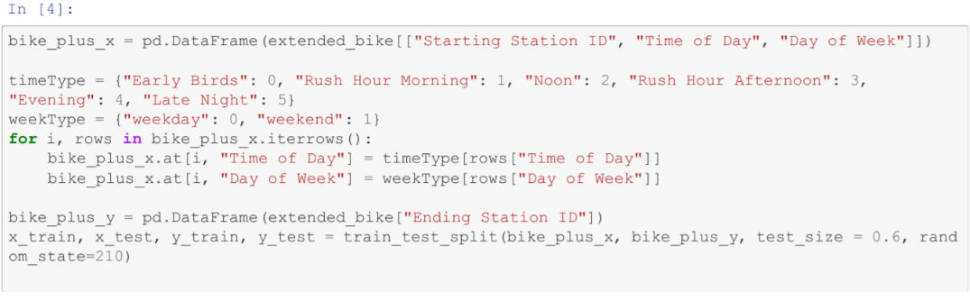
Preparation of the data
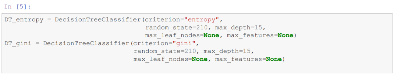
Creating the Decision Tree classifier objects

There are two types of criterias:

These criterias evaluate the data according to its uncertainty depending on its columns. We will focus on entropy in this project, since throughout the semester we used notion of entropy.

Accuracy with entropy: 16.06276819947693

Lets also try with gini to see if there is any difference

Accuracy with gini index: 15.846939034608843

There is no difference between entropy and gini criterias for this case.

Result of this model:

This model is not successful since we can predict final destination with an accuracy of 15%. This result has been achieved after we test our the model on test dataset which is separated from training dataset at the beginning. This is very low. Parameters we had from the datasets were simply not enough to make a reliable prediction. If we could have some user information like age of user, employment status … etc. we could do a better prediction.

2) Duration Prediction by Using Starting Station Crime Rate, Ending Station Crime Rate, Starting Station Accident Rate, Ending Station Accident Rate

Preparation of the data
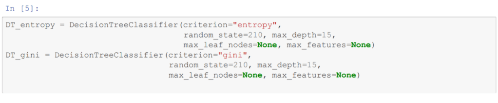
Creating the Decision Tree classifier objects

Again, there are two types of criterias:

We will focus on entropy in this project, since throughout the semester we used notion of entropy.

Accuracy with entropy: 76.3641672802986

Lets also try with gini to see if there is any difference

Accuracy with gini index: 76.3641672802986

The difference between entropy and gini criterias are negligible.

Result of this model:

This model is successful since we can predict ride durations with an accuracy of 76%. We verified that by testing the model on test dataset which is separated from training data. This is high enough to build some models and predict some user behaviour. In this case, we used the fact which we found in Dataset Exploration step. The fact is: how long users ride their bikes is corrolated with crime and accident rates in their area

We tried to visualize the decision tree but due to its large size it was not possible

Support Vector Machine Model

We will use built-in svm function from sklearn

Sklearn is a well known Python library that provides efficient Machine learning algorithms.

A Support Vector Machine (SVM) is a discriminative classifier formally defined by a separating hyperplane. In other words, given labeled training data (supervised learning), the algorithm outputs an optimal hyperplane which categorizes new examples. In two dimentional space this hyperplane is a line dividing a plane in two parts where in each class lay in either side.

In our case space is 2D, therefore our seperation is done by a line into two classes.

Constructing the data that we are going to use for svm

We will use the columns from the extended_bike dataset “Time”, “Starting Station Crime Rate”, “Trip Route Category” By using Time and Starting Station Crime Rate we will try to estimate Trip Route Category. By using Time and Starting Station Crime Rate we will try to estimate Trip Route Category. Which can be one way or round trip.

Preparation of the data

Trip type is given in binary format for the sake of simplicty. Round Trip -> 0 and One Way -> 1

We seperate the data to x (attributes) and y (target variable) parts. Each divided for testing and training purposes.

Sklearn’s built-in svm library does not work with pandas. Thus, we will convert everything to numpy arrays


Dividing the data
Creating the Support Vector Machine classifier object
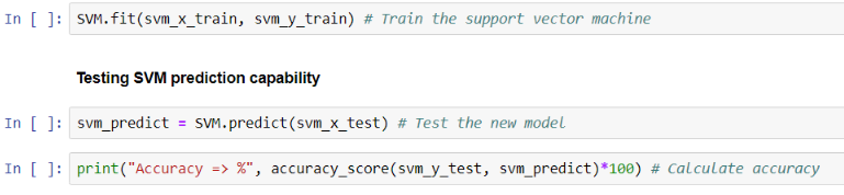
Fitting (training) and testing the model
The accuracy is around 89%

Results:

We have built 3 models to try to estimate 3 different ride features. 2 of them have worked successfully but 1 of them which is the hardest one to predict without user information, has failed. Even so, we are able to create a general profile for every station about their need of bikes. When we want to build a new station, we can predict its required number of bikes for every time slot of the day. Because right now we can predict, if a bike will return to station or how many minutes will the bike be used by taking “Time”, “Starting Station Crime Rate”, “Ending Station Crime Rate”, “Starting Station Accident Rate”, “Ending Station Accident Rate” as inputs.

These two successful prediction models are enough for some simple predictions. The most important part of the project is that we created some features (Crime and Accident Rates for stations) by combining multiple columns and datasets and those features have been successfully used to build a model.

Discussion:

In our three different datasets, we had information columns with various types. At the beginning of the project, in the Data Exploration Phase, we created one big dataset, namely extended_bike, which covers information from our three initial datasets. In this dataset, we were able to reduce the number of type of features to two, namely: discrete classes (e.g. Time Of Day, Starting Station ID… ) and continuous values (Duration, Crime Rates…).

The order of ML Method selection in a normal project should start with Bayesian Decision Tree since it is very easy to implement and very informative in the sense of probability. After that Logistic Regression would be the appropriate choice due to its classification capabilities in continuous space. In order to improve our classification in continuous space, we can use SVM. When we want to switch our continuous feature space to discrete feature space, Decision Trees could give high precision with very small training time.

In our project, we have selected our ML techniques having considered the information we have explained above. Therefore when we use discrete classes for classification, decision tree would be the right choice. On the other hand, when we use continuous data for classification, our model should be SVM due to its continuous space representation capability.

We thought about creating more models but the two successful models gave us enough information to achieve our initial goals. We can predict bike needs fairly accurately for existing or even new stations using time of day, crime rates, and accident rates in the area of the station. Considering this, we decided that adding more models would make the project more complicated than it needs to be. After all, as long as it works, simplicity is better than complexity. There is some more highly correlated information columns which can be predicted by using ML methods. However , those predictions do not help our design goal. Therefore we omitted them.

At the beginning of the project we did some extra research to find more user centred data, however, they were not shared due to privacy concerns. If we would have had user centred data, we could do some analysis about routes and personal pieces of information. So that we could predict some more possible routes along with new locations for possible new stations.

CS210 Final Project Step 2 : Statistical Analysis

https://nbviewer.jupyter.org/gist/oguzhanilter/cf65dde581b67e7a6ea538f6eeba8759

Project Description

In this project, we want to analyse the users of the Los Angeles Metro Bike-Sharing Service and their usage preferences depending on time and locations of the city in order to clarify:

  • Prefered time intervals
  • Effect of crime rate in the area
  • Traffic factor
  • General user statistics

At the end of the project we aim to determine some alternative locations for Bike-Stations based on users’ route preferences.

Used Datasets

We obtained the datasets from Kaggle along with Metro Bikeshare Service official website (https://bikeshare.metro.net/about/data/).

The Crime Dataset contains crime type, place and time in the city. By using the Crime Dataset, we want to obtain general safety profiles of the locations.

Crimes in Los Angeles Dataset has 1584316 rows, and 26 columns. 
Information on every column and their types:
DR Number int64
Date Reported object
Date Occurred object
Time Occurred int64
Area ID int64
Area Name object
Reporting District int64
Crime Code int64
Crime Code Description object
MO Codes object
Victim Age float64
Victim Sex object
Victim Descent object
Premise Code float64
Premise Description object
Weapon Used Code float64
Weapon Description object
Status Code object
Status Description object
Crime Code 1 float64
Crime Code 2 float64
Crime Code 3 float64
Crime Code 4 float64
Address object
Cross Street object
Location object
dtype: object

The Traffic Collision Dataset contains information about traffic accidents such as victim, time, location etc. This is the biggest dataset that we use but most of the accidents are not related to our topics. Therefore this dataset will be downsized by keeping only bike-related accidents.

Traffic Accidents in Los Angeles Dataset has 463819 rows, and 18 columns.
Information on every column and their types:
DR Number int64
Date Reported object
Date Occurred object
Time Occurred int64
Area ID int64
Area Name object
Reporting District int64
Crime Code int64
Crime Code Description object
MO Codes object
Victim Age float64
Victim Sex object
Victim Descent object
Premise Code float64
Premise Description object
Address object
Cross Street object
Location object
dtype: object

Metro Bike Sharing Service Dataset is our main dataset and contains information about every trip defined with the ancillary information about time, location, type of costumer and Bike-Station. Locations of Bike-Stations have been provided both in coordinates and ID of station. A supplementary document contains information about those IDs.

Bike Share Dataset has 132427 rows, and 16 columns.
Information on every column and their types:
Trip ID int64
Duration int64
Start Time object
End Time object
Starting Station ID float64
Starting Station Latitude float64
Starting Station Longitude float64
Ending Station ID float64
Ending Station Latitude float64
Ending Station Longitude float64
Bike ID float64
Plan Duration float64
Trip Route Category object
Passholder Type object
Starting Lat-Long object
Ending Lat-Long object
dtype: object

One problem about the main dataset is, although it contains Los Angeles in the name, the bike-sharing system is applicable only in a small area. Therefore it becomes harder to combine with different datasets as they cover more area and lack detail in area based information.

Center of Crimes and Center of Accidents

City of Los Angeles consists of 21 sub-areas each controlled by different police stations. When the fusion of two datasets (The Traffic Collision in Los Angeles Dataset and The Crime in Los Angeles Dataset) is considered, the number of locations a crime or accident can happen is very big. This makes it very hard to keep track of the effects of every individual crime or accident on the Bike-Sharing Service users’ preferences. Therefore we will create a Center of Crimes and a Center of Accidents for every sub-area.

Substep 1: Pre-Processing

The Traffic Collision in Los Angeles and
The Crime in Los Angeles Datasets.

We will only use a segment of the Traffic Collision Dataset. If we examine the MO Code explanations, there are bike related accidents. We will use only the rows which contain these accidents. The MO Codes are: 0345, 3008, 1223, 3016, 3017, 3018, 3021

The longitude and latitude values were strings in both The Traffic Collision in Los Angeles Dataset and
The Crime in Los Angeles Dataset. So we needed to convert them into integers.

In addition to locations of the Centers, we will need the total number of crime and accidents in the 21 sub-areas. Calculation of Centers is as follows:

We also divided the Time of Day into 6 sections. This way we wont need to deal with continious time series.

Crime Ratio for Time of Day:
Noon 0.343702
Evening 0.281171
Late Night 0.171482
Rush Hour Afternoon 0.106698
Rush Hour Morning 0.067934
Early Birds 0.029013
Name: Time of Day
dtype: float64

Metro Bike Sharing Service Dataset

The time of the day representions does not match between datasets, therefore we will create new columns in order to represent the time in the same format as in The Traffic Collision in Los Angeles Dataset and The Crime in Los Angeles Dataset. In these datasets time is just an integer, which is created in following manner: HHMM. For example 14:02 (2:02 PM) is reprensted as 1402.

In addition to time representation, we will classify the ‘Start Time’ into 6 time of day categories same as the other datasets.

Also we will create a column which represents the day of the week for every trip. However for the sake of simplicity we will classify this information into two categories: Weekday and Weekend.

Weekday    96594 
Weekend 35833

In addition to that, we want to see the locations of the Stations but we can not find that information by using Latitude and Longitude because it does not give enough accuracy.However, we can still use those coordinates to find the distance.

extended_bike[‘distance’] = [geodesic((row[‘Starting Station Latitude’], row[‘Starting Station Longitude’]),(row[‘Ending Station Latitude’], row[‘Ending Station Longitude’])).miles*1.60934 for index,row in extended_bike.iterrows()]

Final Shapes of Datasets

Metro Bike Sharing Service Dataset
New Bike Share Dataset has 131276 rows, and 25 columns
Information on every column and their types:
Trip ID int64
Duration int64
Start Time object
End Time object
Starting Station ID float64
Starting Station Latitude float64
Starting Station Longitude float64
Ending Station ID float64
Ending Station Latitude float64
Ending Station Longitude float64
Bike ID float64
Plan Duration float64
Trip Route Category object
Passholder Type object
Starting Lat-Long object
Ending Lat-Long object
dtype: object
The Traffic Collision in Los Angeles Dataset
New Traffic Dataset has 15976 rows, and 21 columns
Information on every column and their types:
Trip ID int64
Duration int64
Start Time object
End Time object
Starting Station ID float64
Starting Station Latitude float64
Starting Station Longitude float64
Ending Station ID float64
Ending Station Latitude float64
Ending Station Longitude float64
Bike ID float64
Plan Duration float64
Trip Route Category object
Passholder Type object
Starting Lat-Long object
Ending Lat-Long object
dtype: object
The Crime in Los Angeles Dataset. 
New Crime Dataset has 1578834 rows, and 29 columns
Information on every column and their types:
Trip ID int64
Duration int64
Start Time object
End Time object
Starting Station ID float64
Starting Station Latitude float64
Starting Station Longitude float64
Ending Station ID float64
Ending Station Latitude float64
Ending Station Longitude float64
Bike ID float64
Plan Duration float64
Trip Route Category object
Passholder Type object
Starting Lat-Long object
Ending Lat-Long object
dtype: object

Assumption

We will assume that the rate of crime incidents for the region of a Bike-station will be equal to the number of crimes of nearest Center of Crimes divided by distance between The Center of Crimes and that station. Likewise, the rate of traffic accidents will be equal to the number of accidents of nearest Center of Accidents divided by distance. So that we will have the general profile of every Bike-station region.

Substep 2: Data Exploration

In this section we will visualize our datasets and try to create some hypothesis in order to find some correlations between them

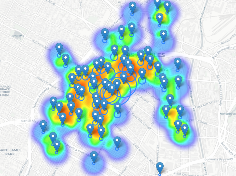
Locations of Bike Stations and Crime Rate Circles :

Heatmap shows the usage of a station. Blue circles around station locations represent Crime rate. Radius of every circle is equal to the Crime Rate of that station.

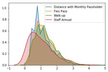
Distance and Pass-Holder Type:

Averae distance for each passholder type

Variation of Average Duration as Time of Day Changes:

Variations of average durations by the time of day

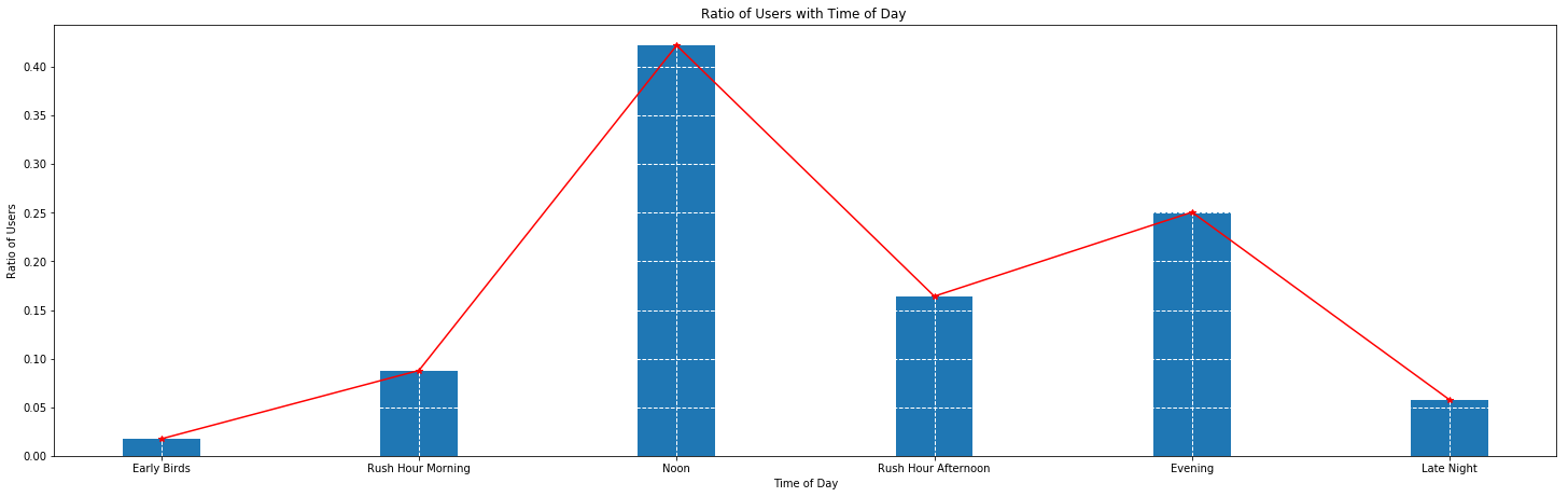
Ratio of Users vs Time of Day:

How the ratio of users is distributed throughout the day

Rate of Crimes vs Time of Day:

How the rate of crimes changes with time of day

Rate of Accidents vs Time of Day:

How the rate of accidents changes with time of day

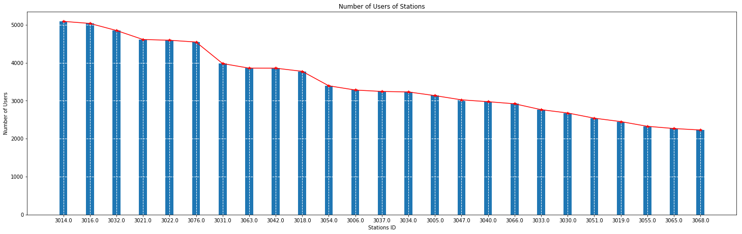
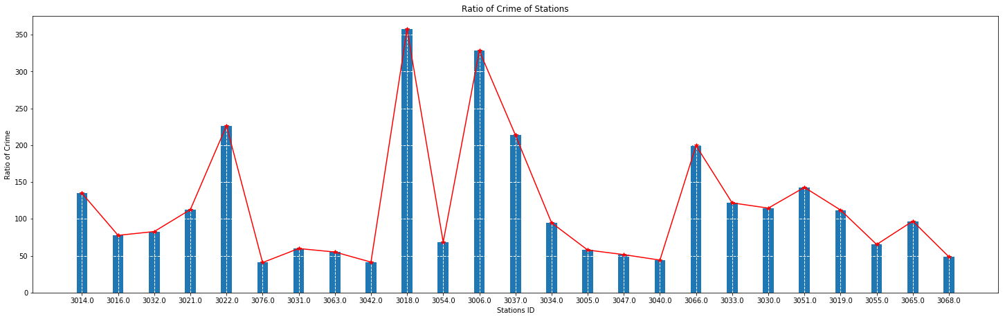
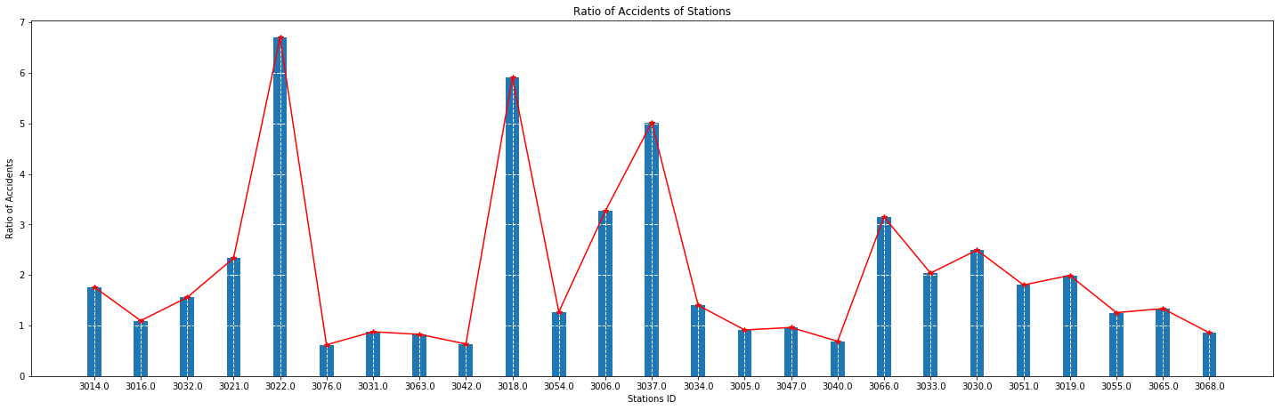
Users, Crime, and Accidents per station:

Number of users for each station
Ratio of crime for each station
Ratio of accidents for each station

Substep 3: Hypothesis Testing

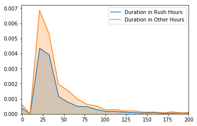
1. Are the long travel times more likely in Rush Hour?

Null Hypothesis (H0) : Longer travels are more likely in Rush Hour.

Result => (statistic=-12.010724249216386, pvalue=3.2488531727977476e-33)

P-value is much lower than 0.05. Therefore we concluded that the null hypothesis is not correct. Longer travels are not more likely in rush hour.

2. Is Pass Holder Type a significant indicator for Long Travelling Distance?

Null Hypothesis (H0) : People with monthly pass go shorter distances because they have a daily routine.

Result => (statistic=-37.68459973577839, pvalue=6.080822547578137e-309)

P-value is much lower than 0.05. Therefore we concluded that the null hypothesis is not correct. People with montly pass does not necessarily go shorter distances.

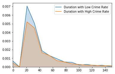
3. Is Long Duration more common in High Crime Areas?

Null Hypothesis (H0) : Areas where people ride bikes for longer times have higher crime rates

Result => (statistic=2.443040040867613, pvalue=0.014565429719958356)

Although the P-value is around 0.01, we will assume that the Null Hypothesis holds. Because the value of Crime Rate is also an assumption for every area. Normally, we would only accept P-values above 0.05 but int his particular case we will accept 0.01.

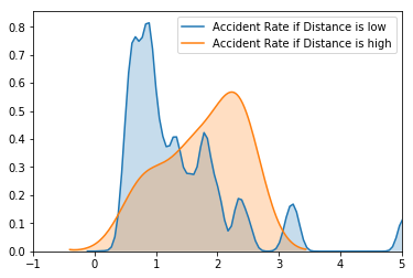
4. Is Long Riding Distance a significant factor for Accident Rate?

Null Hypothesis (H0): The chance of accidents increases as the riding distance gets longer.


Result => (statistic=0.10329975155008089, pvalue=0.917725247586795)

As the P-value is way above 0.05, we can confidently conclude that the Null Hypothesis holds. When people ride for further distances, chance of an accident increases.

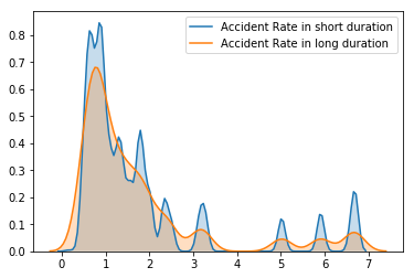
5. Effect of long duration ride on Accident Rate

Null Hypothesis (H0): The chance of accidents increases as the duration gets longer

Result => (statistic=0.8961708866065113, pvalue=0.37016314547529594)

Similar with number 4, the P-value is way above 0.05. We can confidently conclude that the Null Hypothesis holds. When people ride for longer durations, chance of an accident increases.

The Relationship Between Crime Rate and Accident Rate – Linear Regression

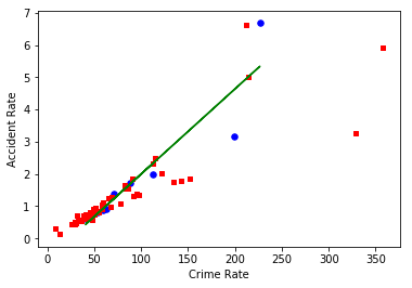
In this part we are asked to build a Linear regression model in order to predict some information in future. Our values are the Crime Rate and Accident Rate. Also by looking this we can conclude that these two values are linearly correlated.

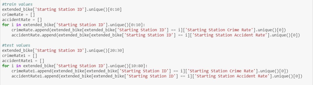
Preperation for the linear regression
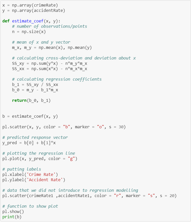
The code for the linear regression model

(-0.6378231281388407, 0.026378162963240314)

The bias of model is -0.6378 and the slope is 0.0263

Proposal of CS210 Group Project

Cities, getting sick of traffic, are more open to innovating away that problem. In our project, we wanted to analyze ‘Bike Sharing’ system, which is a service in which bicycles are made available for shared use to individuals on a short-term basis for a price or free. This system is considered as a solution to traffic problem of crowded cities. However, bike might be problematic for some districts and time of the day in terms of safety issues. In order to analyze the areas from safety point of view, our two additional datasets contain information about traffic accidents and crime records on time and location level with more additional information such as gender and age.

There different datasets will help us to analyze the users of this Bike Sharing system. Their decision about preferred routes might give us general understanding of citizens of Los Angeles how safe they feel when they ride bike on different time and locations. If we can find a correlation between bike routes and crime rates of districts of Los Angeles, we can come up with some new Bike Stops, which would create new routes for users which make them feel more secure on bike ride. This project might help to create more optimal positioning for Bike Stops.

Our datasets:

�T Below some graphs related to our datasets can be found.

Graph about Traffic Accident of Males: Age vs Time of Occurance
Occurence of accidents graphed by Age of the male victims vs. Time of day


Average duration in minutes separated by Passholder types.
The graph on the left is for Round Trips while graph on the right is for One Way Trips

Number of accidents in different areas of the city
Graph on the left is for female bikers while the graph on the right is for male bikers

Average durations plotted by the time of day
The red line is the average duration